Mixed Precision and ZeRO: Training Large Models Without Running Out of Memory

A note on mixed precision, high-precision parameter copies, and ZeRO.

TL;DR

Training large neural networks requires two conflicting desiderata: (1) the speed and memory economy of low-precision compute (FP16 / BF16), and (2) the numerical fidelity of high-precision updates (FP32). The inevitable compromise is to maintain both a high-precision FP32 canonical copy of parameters and a low-precision compute copy; gradients are produced in low precision, then cast to high precision for optimizer arithmetic. When scale forces duplication across devices, ZeRO (Zero Redundancy Optimizer) shards optimizer state, gradients, and — in its strongest form — parameters, trading communication for memory. Below you’ll find the math, the sequence of operations, memory accounting, communication primitives, and some engineering optimizations.

(Frameworks — for example PyTorch and DeepSpeed — implement these ideas in C++/CUDA with many optimizations; the theory here is what they implement under the hood.)

Flow (how to read this note)

1. State the single physical law we are trying to perform.
2. Spell out floating-point mechanics (precision, dynamic range) and why they force a compromise.
3. Give the canonical mixed-precision protocol: FP32 canonical copy, FP16 compute copy, cast gradient, optimizer in FP32, refresh.
4. Account for memory: naive per-device, then data-parallel replication and the urge to shard.
5. Introduce ZeRO: sharding optimizer state (ZeRO-1), gradients (ZeRO-2), and parameters (ZeRO-3).
6. Summarize communication primitives and costs (all-reduce, reduce-scatter, all-gather).
7. Explain why high-precision copies are required (numerical stability, Adam example).
8. Walk through a working ZeRO-1 protocol step by step.
9. List engineering optimizations (bucketing, overlap, prefetch, grad scaling, offload).
10. Give some practical recipes.
11. Note common failure modes.
12. Close with the ledger metaphor.

Prelude — the single physical law

There is only one true operation we are trying to perform:

where $\theta\in\mathbb{R}^N$ is the full parameter vector and $\Delta(\theta)$ is the update computed by your optimizer (for SGD $\Delta=\nabla\mathcal{L}$; for Adam it is a more elaborate function of past gradients). Computers approximate reals with floating point. That approximation imposes constraints that force the whole engineering stack you now know exists.

Floating-point mechanics

Floating point numbers are finite encodings of real numbers. IEEE-754 binary formats represent a number as:

where $s$ is the sign bit, $e$ the exponent field, $b$ the bias, and $m$ the significand bits. Two consequences matter for training:

1. Precision (significand length). FP16 has 10 significand bits (≈3 decimal digits); BF16 preserves the wider exponent range of FP32 but with fewer significand bits; FP32 has 23 significand bits (≈7 decimal digits).
2. Dynamic range (exponent). BF16 and FP32 share greater exponent range than FP16; overflow/underflow behavior depends on exponent fields.

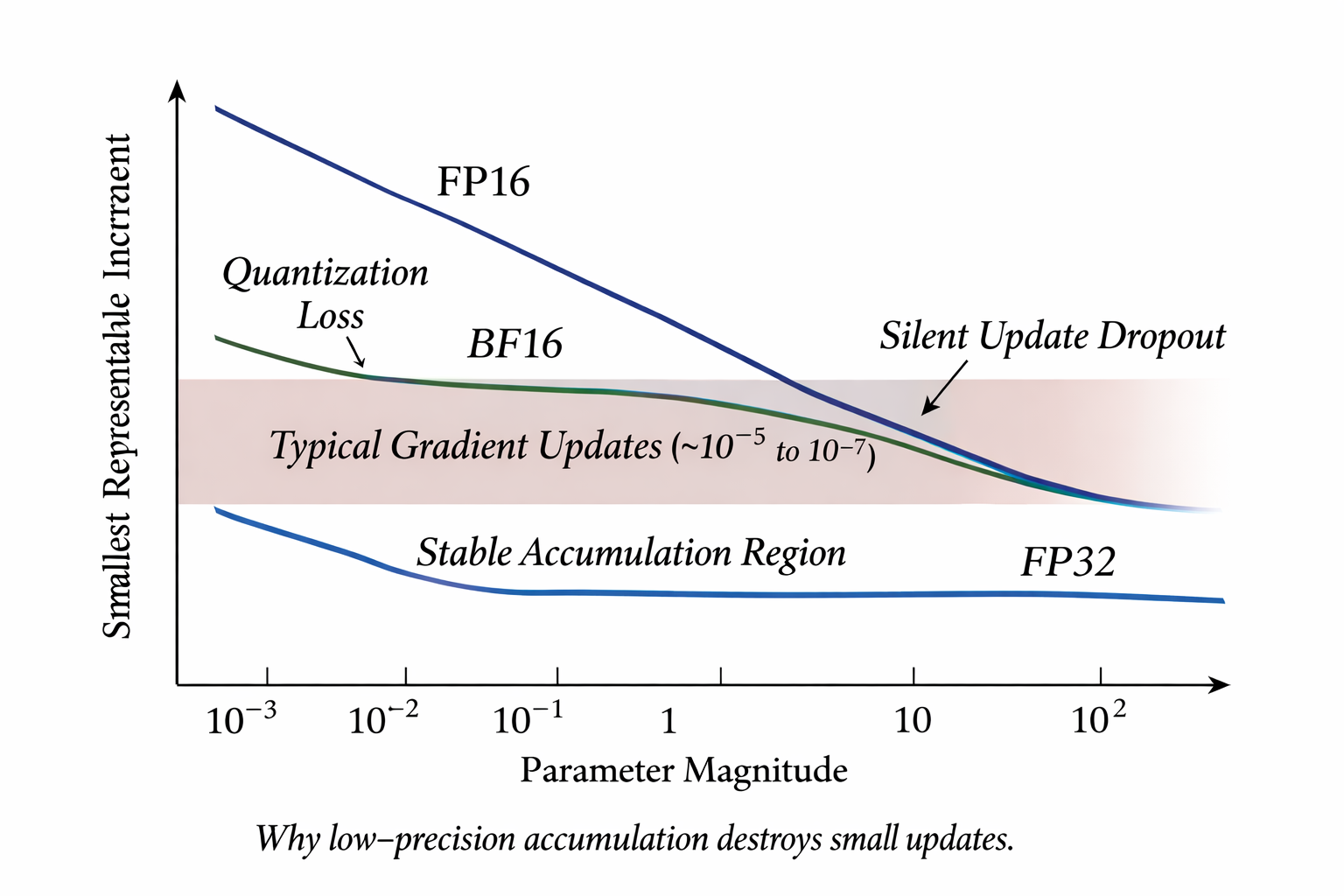
Implication for updates. If $\theta \approx 1.0$ and the update $\delta\theta \approx 10^{-5}$, FP16 may not represent $\delta\theta$ when added to $\theta$ — the result rounds back to $\theta$. Thus, performing repeated incremental updates in low precision leads to loss of meaningful progress.

The canonical mixed-precision protocol (exact sequence)

From the physical constraints above, the robust protocol used in modern training is:

1. Maintain a high-precision FP32 canonical parameter copy $\theta^{(32)}$ (FP32). This is the authoritative value.
2. Maintain a low-precision compute copy $\theta^{(16)} = \operatorname{cast}_{16}(\theta^{(32)})$ (FP16 or BF16) used in forward/backward.
3. During backward, compute low-precision gradients $\nabla_{\theta^{(16)}} \mathcal{L}$ (initially FP16/BF16).
4. Convert gradients to FP32: $\nabla^{(32)} = \operatorname{cast}_{32}(\nabla^{(16)})$.
5. Perform optimizer arithmetic in FP32 updating $\theta^{(32)}$ (and optimizer state like moments $m,v$ in FP32).
6. Refresh compute copy: $\theta^{(16)} \leftarrow \operatorname{cast}_{16}(\theta^{(32)})$.

In symbolic form:

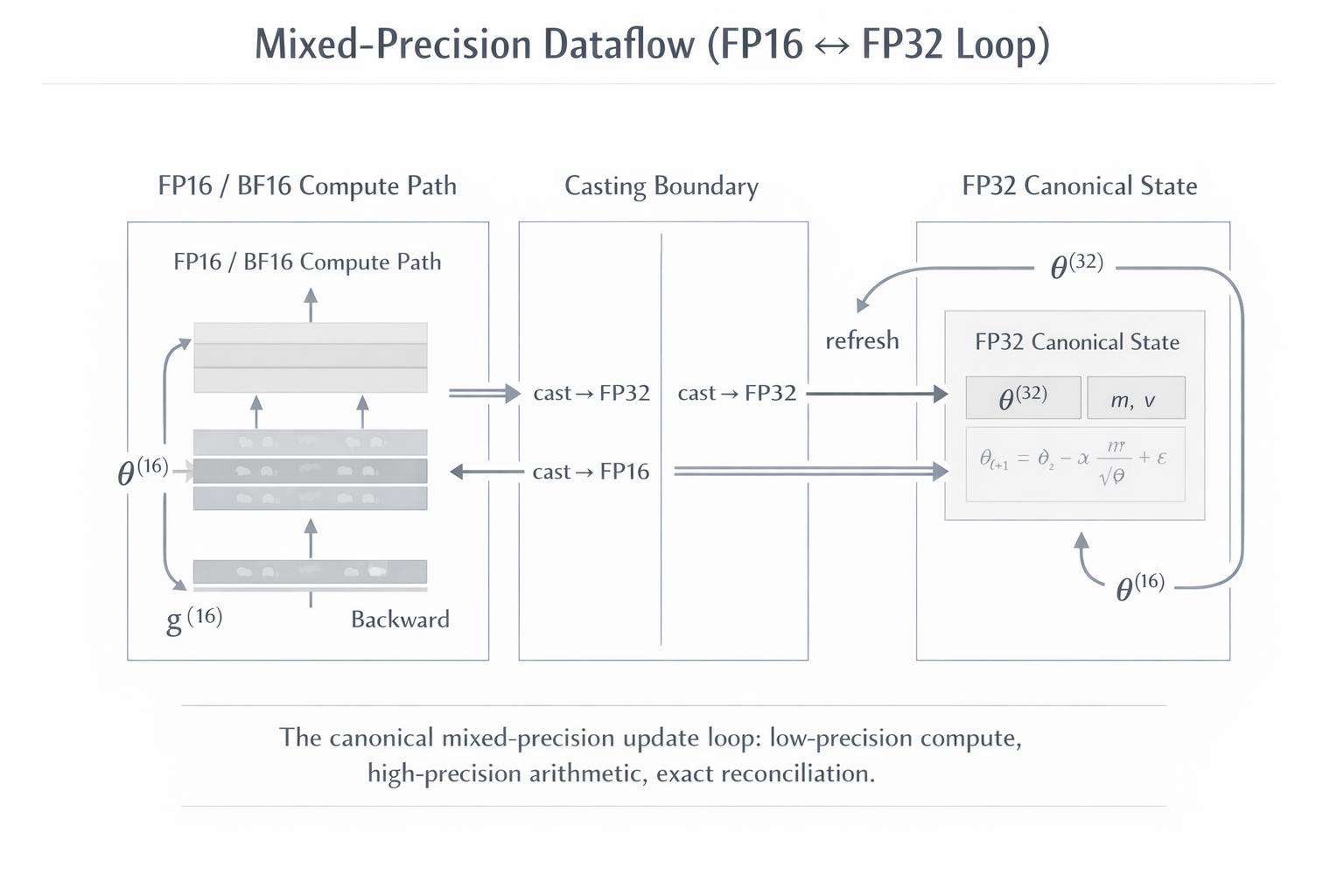
Why both copies? Because the optimizer math requires the dynamic range and precision of FP32 to preserve small incremental updates and accumulated moments; the compute path benefits from the throughput of low precision on modern tensor cores.

Memory accounting

Let $\Psi$ denote the number of scalar parameters. Let element sizes be $s_{16}$ and $s_{32}$ bytes (2 and 4 bytes). Let $k$ denote the optimizer multiplier: the number of parameter-sized FP32 tensors the optimizer keeps (for Adam with FP32 canonical copy, $k\approx 3$: exp_avg, exp_avg_sq, FP32 canonical copy; retain symbolic $k$ for clarity).

Naive per-device memory (single replica, no sharding):

• FP16 parameters: $s_{16}\Psi$
• FP32 canonical weights: $s_{32}\Psi$
• Optimizer states: $k\cdot s_{32}\Psi$
• Gradients (peak): ≈ $s_{16}\Psi$ before casting, then $s_{32}\Psi$ (short lived)

So peak model-related memory (ignoring activations) is roughly:

Plugging $s_{16}=2$, $s_{32}=4$ and $k\approx 2$ yields a concrete feeling: per parameter ≈ $2 + 4 + 8 = 14$ bytes. For billion-parameter models this becomes terabytes.

Data-parallel replication. If you replicate the above across $N_d$ data-parallel devices, you multiply the model-related memory by $N_d$. Thus the urgency to shard.

ZeRO

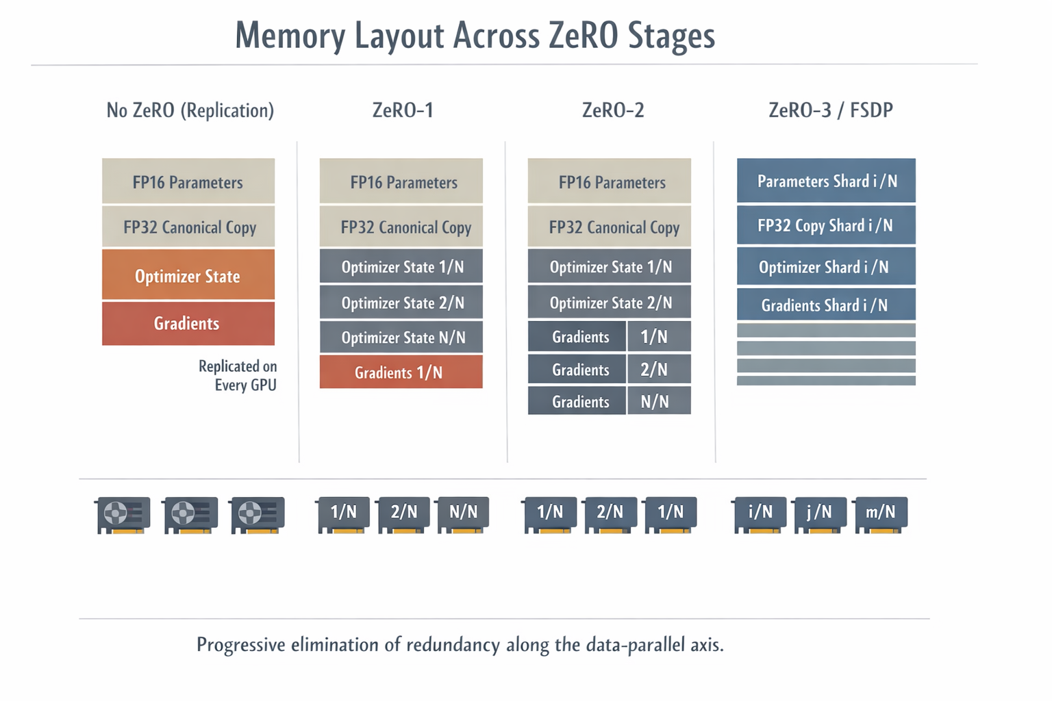
ZeRO shards along the data-parallel axis to remove redundancy. Let $N_d$ be DP degree.

Define three boolean indicators whether an object is sharded: $S_p$ for parameters, $S_g$ for gradients, $S_o$ for optimizer state. If an object is sharded, its contribution to per-rank memory divides by $N_d$.

Per-rank model memory (excluding activations) is:

where $\alpha$ encodes whether gradients are kept as FP16 then cast or kept in FP32 (use $\alpha=1$ for FP32 grad accumulation). We can simplify for common cases.

ZeRO-1 (optimizer state sharded)

$S_o=1$, $S_g=0$, $S_p=0$.

Per-rank memory:

Interpretation: parameters and gradients still replicated; only optimizer state is sharded.

ZeRO-2 (optimizer state + gradients sharded)

$S_o=1$, $S_g=1$, $S_p=0$.

Per-rank memory:

Here gradient and optimizer state both scale down by $1/N_d$.

ZeRO-3 (full sharding; parameters also sharded; a.k.a. FSDP)

$S_o=1$, $S_g=1$, $S_p=1$.

Per-rank memory:

As $N_d$ grows, the model-related memory per rank can shrink arbitrarily (activations remain unsharded unless other techniques are applied).

Note about activations. Activation memory does not replicate across DP ranks — activations differ per micro-batch. Thus ZeRO cannot reduce activation memory; use activation checkpointing or sequence/batch strategies to reduce activation footprint.

Communication primitives and costs

Three collectives matter:

• All-reduce: every rank gets the fully reduced tensor. Cost roughly $2\times$ size network traffic (reduce + broadcast) in classical implementations; efficient implementations reduce constants.
• Reduce-scatter: performs reduction and scatters shards so each rank receives one shard of the reduced result. It is cheaper than all-reduce when you only need shards.
• All-gather: every rank sends its shard and every rank receives the full concatenation.

ZeRO replaces an all-reduce on gradients (vanilla DP) with a reduce-scatter + local update + all-gather on parameters (ZeRO-1/2), or with continuous layerwise all-gathers during forward/backward (ZeRO-3).

Communication complexity per step (measured in parameter-sized data transferred) — denote $|\Psi|$ as the size:

• Vanilla DP: gradients all-reduce cost ≈ $2\Psi$.
• ZeRO-1/2: reduce-scatter gradients cost ≈ $\Psi$ (distributed), plus an all-gather of parameters cost ≈ $\Psi$; total ≈ $2\Psi$ but the pattern and overlap differ and memory pressure is substantially reduced.
• ZeRO-3: parameters are all-gathered layerwise — roughly $3\Psi$ of communication tax if done naively, but overlap/prefetching and grouping reduce wall-time overhead.

Latency vs bandwidth trade. Many small collectives incur latency; bulked transfers favor bandwidth. Engineering thus buckets parameters to balance per-call latency and per-byte throughput.

Precise numerical stability mechanics: why high-precision copies are required

Consider one scalar parameter $\theta \sim 1.0$ and an update $\delta = 10^{-5}$. In floating point:

• FP16 spacing near 1.0 is $2^{-10}\approx 9.8\times 10^{-4}$ — updates of $10^{-5}$ vanish.
• FP32 spacing near 1.0 is $2^{-23}\approx 1.2\times 10^{-7}$ — updates of $10^{-5}$ are preserved.

Thus to preserve the iterative accumulation of small updates, optimizer accumulation (moment estimates, bias corrections) must be maintained in FP32. Storing only FP16 copies will catastrophically quantize the update loop.

Adam example (exact): Adam update for parameter $i$ at step $t$:

Each of $m_t$, $v_t$, $\hat{m}_t$, $\hat{v}_t$ benefits from FP32 precision to avoid bias amplification and catastrophic cancellation; casting them to FP16 would destroy the algorithm’s internal fidelity.

A Working Protocol for ZeRO-1

Below is the precise step performed on each DP rank for ZeRO-1: optimizer-state sharding while parameters remain replicated in FP16.

1. Keep $\theta^{(16)}$ (full, local) and $\theta^{(32)}_{\text{shard}}$, $m_{\text{shard}}$, $v_{\text{shard}}$ (sharded FP32 canonical pieces).

2. For a minibatch:

   • forward using $\theta^{(16)}$.
   • backward producing local $g^{(16)}$.
   • flatten and pad $g^{(16)}$ to common size; compute reduce-scatter → receive gradient shard $g_{\text{shard}}^{(\text{sum},16)}$.
   • cast $g_{\text{shard}}^{(\text{sum},32)} = \operatorname{cast}_{32}(g_{\text{shard}}^{(\text{sum},16)})$ and divide by $N_d$ if gradients are averaged.
   • update local optimizer state and $\theta^{(32)}_{\text{shard}}$ using Adam formulas above.
   • cast local updated $\theta^{(32)}_{\text{shard}}$ to FP16 → $\hat{\theta}^{(16)}_{\text{shard}}$.
   • all-gather $\hat{\theta}^{(16)}_{\text{shard}}$ → reconstruct full $\theta^{(16)}$ on each rank for next forward.
   • zero gradients / manage buffers.

This sequence preserves mathematically identical parameter updates to the naive single-device FP32 update, up to floating point rounding differences introduced by different reduction order — which are typically negligible if using stable reduction algorithms.

Engineering optimizations

Some engineering levers that matter:

• Bucketed communications. Aggregate small tensors into buckets sized to saturate NIC bandwidth to amortize latency.
• Non-blocking collectives + overlap. Launch reduce-scatter as soon as a bucket’s gradients are ready (backward hooks). Launch parameter all-gathers as soon as a shard’s update is ready (optimizer step) and overlap with remaining optimizer computation.
• Prefetching in ZeRO-3/FSDP. While computing layer $n$'s forward, prefetch (all-gather) parameters for layer $n+1$.
• Meta device construction. Build architecture shapes on device=meta to avoid materializing full parameter tensors before sharding (saves memory on initialization).
• Grad scaling (AMP). Multiply loss by a scale $S$ to avoid FP16 overflow; unscale gradients before optimizer step and detect inf/nan to adjust $S$.
• Offload. When device RAM is insufficient, offload rarely used optimizer state shards to CPU or NVMe with asynchronous I/O, overlapping transfers with compute.
• Checkpoint sharding. Save sharded state dicts; avoid gathering full parameter sets to a single node for checkpoint writes.

Practical recipes

A production checklist, from smallest to largest scale:

1. Use AMP (autocast + GradScaler). Prefer BF16 on hardware that supports it if you can eliminate GradScaler safely.
2. Use FSDP / ZeRO (library implementation) rather than writing manual sharding. Let the runtime handle hooks and bucketization.
3. Combine ZeRO-2 / ZeRO-3 with activation checkpointing and gradient accumulation when activations are the bottleneck.
4. Use per-layer prefetching and sensible FSDP unit sizes (don’t shard at too fine granularity).
5. Profile: measure collective sizes, time spent waiting on NCCL, and memory peaks; tune bucket sizes and prefetch windows.
6. Ensure deterministic reduction order only if you need bitwise reproducibility; otherwise prefer throughput-optimized reductions.

Common failure modes

• Loss explosion / NaNs. Often caused by overflow in FP16 matmuls. Grad scaling prevents this: multiply loss by $S$, compute gradients, then divide by $S$ before updating.
• Stalled training (no progress). Often caused by updates being lost to quantization if you tried to update exclusively in FP16. The theory above shows why a high-precision FP32 canonical copy is required.
• Excessive communication overhead. Happens when bucket sizes are too small: latency dominates. The communication model above explains why aggregating transfers increases effective bandwidth.
• Activation OOM even with ZeRO-3. ZeRO reduces model-related memory, not activations; employ checkpointing and accumulation to reduce activation peaks.

Closing remark

• FP32 canonical copy = the ledger in the bank. It is the canonical truth, carefully recorded.
• FP16 compute copy = the working checkbook. You do the arithmetic quickly here and then reconcile with the ledger.
• ZeRO sharding = splitting the ledger’s pages across vaults. Each vault keeps its pages and returns photocopies when needed.